Believe those who are seeking the truth. Doubt those who find it. Andre Gide

Wednesday, December 31, 2014

Brad DeLong on the Employment-to-Population Rate

Brad DeLong offers his musing here on the U.S. employment-to-population rate. As a rough control for demographic factors, he focuses on prime-age workers--those aged between 25-54. And he decomposes prime-age workers by sex. I like this exercise. In fact I've looked at the same data in an earlier post here, making comparisons with Canada. 

DeLong normalizes the E-P rate for males and females to zero in the year 2000. For both sexes, the E-P rate is roughly 5% lower than in 2000. Here is his graph:


In reference to this data, DeLong asks a few questions. Heck, it's the end of the year and I'm in the mood to answer some of them.
(1) If the US economy were operating at its productive potential, the share of 25 to 54-year-olds who are employed ought to be what it was at the start of 2000. Back then there were few visible pressures leading to rising inflation in the economy.
Does anybody disagree with that?
I'm not sure, so I think I'll disagree. It's very hard, I think, to know precisely what constitutes "productive potential." And the use of the word "potential" leads us (possibly incorrectly) to interpret the deviations in the graph above as "cyclical" (mean-reverting) fluctuations. I think that some of the decline in the male E-P rate can be reasonably thought of as being "below potential." I base my assessment on this graph (which I plotted a year ago and uses the 16+ population as a base):


This longer time-series shows a modest secular decline in the E-P ratio in both the U.S. and Canada since 1976. Personally, I think it's unlikely that the local peak in 2000 represents some magical measure of "potential." My hunch is that there are "structural" factors at play here including, but not limited to, things like rising disability rates. Having said this, I also don't believe that the male E-P rate has fully recovered. As I've mentioned before, the current dynamic resembles very much what Canada went through in the 1990s, i.e.,


The idea that the female E-P ratio is far below "potential" is even more misleading, I think. There's something strange going on with U.S. female employment relative to other advanced countries (all which resemble Canada in the diagram below).


Again, it's likely that a part of the post-2008 decline is cyclical. But its even more likely that most of the decline is structural (e.g., changing maternity leave benefits, etc.). My own feeling is that structural issues are better tackled through fiscal (or labor market) policies--not monetary policy.
(3) Even if you think–in spite of the absence of accelerating inflation–that employment in 2000 was above the economy’s long-term sustainable potential, there is no reason to believe that a U.S. economy firing on all cylinders would not have 25-54 employment to population rates–both male and female–back at their 2006 levels, a full 3%-age points–and 4%, 1/25–higher than today.
Does anybody disagree with that?
I'm not going to disagree with this.
(4) The U.S. economy’s convergence towards its potential is very slow: The 25-54 employment-to-population ratio has only risen by 1%-point over the past two years.
Does anybody disagree with that?
I'm not going to disagree with this either. However, my interpretation of this phenomenon is a "structural" one, which I explain here (see also here).
(5) Yet in spite of all these, the Federal Reserve believes that the U.S. economy is now close enough to its productive potential that unless some more things go wrong it is no longer appropriate for it to be buying assets and it will be appropriate for it in a year to start raising interest rates even though inflation is still below its 2%/year target.
Well, I'm not speaking for the Fed here (and remember, there are divergent views within the FOMC), but the consensus view seems to be that inflation is just "temporarily" below target. And the recent FOMC statement makes clear that any rate hike will be made contingent on the incoming data. Moreover, even if a rate hike is in the making, it is likely (in my view) to be described as progressing at a "measured pace," similar to the way it was in 2004.
The only way to square (1) through (4) with (5) is if the Greater Crash of 2008-2009 and the still-ongoing Lesser Depression really have pushed between 2 and 4%-age points of our 25 to 54-year-olds out of the labor force permanently, so that we can never get them back, or at least never get them back without an economy at such high pressure to produce inflation that the Federal Reserve regards as unacceptable.
Yes, I suppose this is just another way of saying that a major component of the decline in the E-P rates reported above are attributable to "structural" factors that are better dealt with (if at all) with fiscal policy.
This may be true.
But it does raise two questions: 
[1] What has made the Federal Reserve so confident that it is true that it is willing to make policy based on it–especially as current inflation is still below the 2%/year target?
Again, I am not speaking for the Fed here. But one argument I often hear is that additions to the Fed's balance sheet have not been very effective, especially in terms of improving the labor market. At the same time, people have expressed some degree of nervousness over "not knowing what they don't know" about operating with such a large balance sheet. The Fed is charting new territory here. The benefits seem small at best, and the risks are not fully known. There is some concern that a low-rate policy may induce a "reaching for yield phenomena," leading to financial instability.

Yes, inflation is still below the 2% target, but not that much below. Does a 1.5% inflation rate warrant a policy rate of 25 basis points? Historical Taylor rules evidently suggest that a higher (but still low) policy rate is desirable in the present circumstances. (Note, once again, this is not necessarily my own view.)
[2] If it is true that the missing 2 to 4%-age points of 25 to 54-year-olds now out of the labor force could not be pulled back in without allowing inflation to rise above it’s 2%/year target, isn’t that an argument for raising the 2%/year target rather than accepting the current 77% 25-54 employment to population ratio as the economy’s limit of potential?
No, I don't think raising the long-run inflation target (to say 3% or 4%) will have any measurable long-run impact on the labor market. A significantly higher inflation tax may even discourage employment (the long-run Philips curve may be positively sloped). If there are things that need "fixing" in the labor market six years into the recovery, they are probably better dealt with directly through labor market policies (like improved maternity leave benefits) or fiscal policies (tax cuts, wage/training subsidies, etc.)

***
Some background reading: Many Moving Parts: A Look Inside the U.S. Labor Market.

Thursday, December 18, 2014

Considerable Time and Patience a Decade Ago

According to USA Today:
Wall Street cheered as the Federal Reserve used a new word — "patient" — to basically let the market know that it isn't in a rush to hike short-term rates next year.
So, "patient" is the new buzzword. In other words, the Fed evidently ran out of patience with "considerable time." 

But just how new are these buzzwords? They're not new at all. Consider this from the December 09, 2003 FOMC statement, for example.
However, with inflation quite low and resource use slack, the Committee believes that policy accommodation can be maintained for a considerable period.
This "considerable period" language was also used in the August 12, September 16, and October 28 FOMC statements leading up to the December statement. The FF target rate at that time was 1%. Headline PCE inflation was running at about 2% (year-over-year), and the unemployment rate was about 5.5%.

Then, at the next FOMC meeting, the Fed switched from "considerable period" to "patient." From the January 28, 2004 FOMC statement
With inflation quite low and resource use slack, the Committee believes that it can be patient in removing its policy accommodation.
Note that "inflation quite low" in January 2004 was 2%. The FOMC continued to express "patience" in its March 16 statement. In its May 4 statement, "patience" was replaced with:
At this juncture, with inflation low and resource use slack, the Committee believes that policy accommodation can be removed at a pace that is likely to be measured.
Note that the "with inflation still low" statement now corresponds to PCE inflation running around 2.5%. 

It wasn't until the June 30 statement that the FOMC finally raised the FF target rate by 1/4%. And for the next 17 meetings, the FOMC raised its policy rate by 25 basis points. 

Should the Fed at that time exhibited less patience, both in the the timing and pace of "lift off?" Certainly John Taylor seems to think so

And what about the situation today? While the unemployment rate today (5.8%) is not far from where it was eleven years ago, the policy rate is at 1/4% (instead of 1%) and the PCE inflation rate is at 1.5% (instead of 2%). At the risk of oversimplifying, there are basically two views on the matter.

The dovish argument is that with inflation and inflation expectations low (relative to target) and unemployment still elevated somewhat, keeping the policy rate at its floor seems like the right thing to do right now. What this has to do with "considerable time" or "patience," I'm not sure. It is a state-contingent policy. (Adding "considerable time" or "patience" to the statement simply reveals the FOMC's own assessment of the probabilities associated with future states of the world.)

The hawkish argument is that the real economy is basically back to normal, that while inflation and inflation expectations are currently low, this is largely transitory. And in any case, the welfare cost/benefit of 1.5% inflation vs. 2% inflation is virtually nil. So, with inflation and unemployment at close to normal levels, why shouldn't the policy rate also start moving closer to normal levels? (There are also other concerns relating to low interest rates and financial instability--look at what happened the last time we had a "patient" Fed.) 

Stay tuned, folks.

Thursday, November 27, 2014

Bitcoiners: Surely we can do Buiter than this?

Willem Buiter has a very nice piece critiquing the Swiss Gold Initiative; see here.

Unfortunately, Buiter starts talking about Bitcoin, making false analogies between the cryptocurrency and gold. He should have just focused on gold.

As it turns out, both gold and Bitcoin do share some important characteristics. I've written about this here: Why Gold and Bitcoin Make Lousy Money.

The false analogy is in equating the mining of gold with the mining of bitcoin. Paul Krugman made the same mistake here: Adam Smith Hates Bitcoin. Here is the offending passage in Buiter's notes:
John Maynard Keynes once described the Gold Standard as a “barbarous relic”. From a social perspective, gold held by central banks as part of their foreign exchange reserves merits the same label, in our view. The same holds for gold held idle in private vaults as a store of value. The cost and waste involved in getting the gold out of the ground only to but it back under ground in secure vaults is considerable. Mining the ore is environmentally damaging, especially if it involves open pit mining. Refining the gold causes further environmental risks. Historically, gold was extracted from its ores by using mercury, a toxic heavy metal, much of which was released into the atmosphere. Today, cyanide is used instead. While cyanide, another toxic substance, is broken down in the environment, cyanide spills (which occur regularly) can wipe out life in the affected bodies of water. Runoff from the mine or tailing piles can occur long after mining has ceased. 
Even though, from a social efficiency perspective, the mining of new gold and the costly storage of existing gold for investment purposes are wasteful activities, they may be individually rational. The same applies to Bitcoin. Its mining is socially wasteful and environmentally damaging.
No, no, no and no. This analogy is all wrong.

Let me be clear about this. Bitcoin costs zero to produce. If one had control over the protocol, one could instantly and costlessly create as many bitcoins as one wanted. No environmental waste, no effort needed. The same is not true of gold.

But wait a minute, you might say. Doesn't mining for bitcoins require effort, consume resources, etc.? The answer is, yes, it does. But this fact does not make the analogy correct (though one can certainly understand why the analogy seems to be correct). Let me explain.

The purpose of gold miners is to prospect for gold. The purpose of Bitcoin miners is not to prospect for bitcoins. The purpose of Bitcoin miners is to process payment requests. A bank teller also processes payment requests. To say that miners are mining for bitcoin is like saying that tellers are mining for dollars. Understand? Let me try again.

Gold miners prospect for gold. But they do not necessarily get paid in gold. In fact, if they work for gold companies, they are likely to get paid in dollars. But they could get paid in gold, or anything else, for that matter. How they get paid does not take away their basic function, which is to discover new gold.

Bitcoin miners, like bank tellers, process payments. Miners, like tellers, want to get paid for the service they provide. It really does not matter how they are paid. As it turns out, miners are paid in the form of newly-issued bitcoins (as well as old bitcoins offered as service fees by transactors). But this does not mean that they are "mining for bitcoin" any more than a bank teller is "mining for dollars."

But isn't mining for bitcoin "wasteful?" In a sense, yes, but again, the "waste" here is not the same as the waste associated with commodity money. Again, let me explain.

We live in a "second-best" world, where people lie and cheat. In a first-best world, money would not even be necessary (see my post here: Evil is the Root of All Money). It is unfortunate that we need Bitcoin miners (and tellers) to process payments. But the resources consumed in this process are necessary, given the safeguards that have to enforced to ensure the integrity of the payment system.

The waste associated with mining gold is that in principle, gold money can be replaced by paper money (and please, do not give some weird "out of thin air" argument; see here.) Paper money, like Bitcoin, and unlike gold, is (near) costless to produce.

Note: Of course, the limit on the supply of bitcoin is determined by a community consensus on following the protocol that adopts the 21M limit. Bitcoin advocates argue that this "hardwired" protocol that governs the supply of bitcoin is more reliable and less prone to political manipulation relative to existing central banking systems. This all may be true, but does not take away from my argument above concerning the false analogy between gold and bitcoin.


Tuesday, November 18, 2014

Japan: Some Perspective

So Japan is in recession.  And it's all so unexpected. Ring the alarm bells!

Well, hold on for a moment. Take a look at the following diagram, which tracks the Japanese real GDP per capita since 1995 (normalized to equal 100 in that year). I also decompose the GDP into its expenditure components: private consumption, government consumption, private investment, and government investment (I ignore net exports). The GDP numbers go up to the 3rd quarter, the other series go up to only the 2nd quarter.


In terms of what we should have expected, I think it's fair to say that most economists would have predicted the qualitative nature of the observed dynamic in response to an anticipated tax hike. That is, we'd expect people to substitute economic activity intertemporally--front loading activity ahead of the tax hike, then curtailing it just after. And qualitatively, that's exactly what we see in the graph above. But does the drop off in real per capita GDP really deserve all the attention it's getting? I don't think so. The fact that the economy was a little weaker in the 3rd quarter than expected (the two consecutive quarters of GDP contraction is what justified labeling the event a "recession") is not really something to justify wringing one's hand over. Not yet, at least.

By the way, if you're interested in reading more about the Koizumi boom era, see my earlier post here: Another look at the Koizumi boom.

Saturday, November 15, 2014

Roger Farmer on labor market clearing.

While I'm a huge fan of Roger Farmer's work, I think he gets this one a little wrong:  Repeat After Me: The Quantity of Labor Demanded is Not Always Equal to the Quantity Supplied. I am, however, sympathetic to the substantive part of his message. Let me explain.

The idea of "supply" and "demand" is rooted in Marshall's scissors (a partial equilibrium concept). The supply and demand framework is an extremely useful and powerful way of organizing our thinking on a great many matters. And it is easy to understand. (I have a pet theory that if you really want to have an idea take hold, you have to be able to represent it in the form of a cross. The Marshallian cross. The Keynesian cross. Maybe even the Christian cross.)

The Marshallian perspective is one in which commodities are traded on impersonal markets--anonymous agents trading corn and human labor alike in sequences of spot trades. Everything that you would ever need to buy or sell is available (absence intervention) at a market-clearing price. The idea that you may want to seek out and form long-lasting relationships with potential trading partners (and that such relationships are difficult to form) plays no role in the exchange process--an abstraction that is evidently useful in some cases, but not in others.

I think what Roger means to say is that (repeat after me) the abstraction of anonymity, when describing the exchange for labor services, is a bad one. And on this, I would wholeheartedly agree (I've discussed some of these issues in an earlier post here).

Once one takes seriously the notion of relationship formation, as is done in the labor market search literature, then the whole concept of "supply and demand" analysis goes out the window. That's because these well-defined supply and demand schedules do not exist in decentralized search environments. Wage rates are determined through bargaining protocols, not S = D. To say, as Roger does, that demand does not always equal supply, presupposes the existence of Marshall's scissors in the first place (or,  more generally, of a complete set of Arrow-Debreu markets).

And in any case, how can we know whether labor markets do not "clear?" The existence of unemployment? I don't think so. The neoclassical model is one in which all trade occurs in centralized locations. In the context of the labor market, workers are assumed to know the location of their best job opportunity. In particular, there is no need to search (the defining characteristic of unemployment according to standard labor force surveys). The model is very good at explaining the employment and non-employment decision, or how many hours to work and leisure over a given time frame. The model is not designed to explain search. Hence it is not designed to explain unemployment. (There is even a sense in which the neoclassical model can explain "involuntary" employment and non-employment. What is "involuntary" are the parameters that describe an individuals' skill, aptitude, etc. Given a set of unfortunate attributes, a person may (reluctantly) choose to work or not. Think of the working poor, or those who are compelled to exit the labor market because of an illness.)

Having said this, there is nothing inherent in the neoclassical model which says that labor market outcomes are always ideal. A defining characteristic of Rogers' work has been the existence of multiple equilibria. It is quite possible for competitive labor markets to settle on sub-optimal outcomes where all markets clear. See Roger's paper here, for example.

The notion that supply might not equal demand may not have anything to do with understanding macroeconomic phenomena like unemployment. I think this important to understand because if we phrase things the way Roger does, people accustomed to thinking of the world through the lens of Marshall's scissors are automatically going to look for ways in which the price mechanism fails (sticky wages, for example). And then, once the only plausible inefficiency is so (wrongly) identified, the policy implication follows immediately: the government needs to tax/subsidize/control wage rates. In fact, the correct policy action may take a very different form (e.g., skills retraining programs, transportation subsidies, job finding centers, etc.)

Monday, November 10, 2014

A dirty little secret


Shhh...I told you *nothing!* 
There's been a lot of talk lately about the so-called "Neo-Fisherite" proposition that higher nominal interest rates beget higher inflation rates (and vice-versa for lower nominal interest rates). I thought I'd weigh in here with my own 2 cents worth on the controversy.

Let's start with something that most people find uncontroversial, the Fisher equation:

[FE]  R(t) = r(t) + Π (t+1)

where R is the gross nominal interest rate, r is the gross real interest rate, an Π is the expected gross inflation rate (all variables logged).

I like to think of the Fisher equation as a no-abitrage condition, where r represents the real rate of return on (say) a Treasury Inflation Protected Security (TIPS) and (R - Π) represents the expected real rate of return on a nominal Treasury. If the two securities share similar risk and liquidity characteristics, then we'd expected the Fisher equation to hold. If it did not hold, a nimble bond trader would be able to make riskless profits. Nobody believes that such opportunities exist for any measurable length of time.

Let me assume that the real interest rate is fixed (the gist of the argument holds even if we relax this assumption). In this case, the Fisher equation tells us that higher nominal interest rates must be associated with higher inflation expectations (and ultimately, higher inflation, if expectations are rational). But association is not the same thing as causation. And the root of the controversy seems to lie in the causal assumptions embedded in the Neo-Fisherite view.

The conventional (Monetarist) view is that (for a "stable" demand for real money balances), an increase in the money growth rate leads to an increase in inflation expectations, which leads bond holders to demand a higher nominal interest rate as compensation for the inflation tax. The unconventional (Neo-Fisherite) view is that lowering the nominal interest leads to...well, it leads to...a lower inflation rate...because that's what the Fisher equation tells us. Hmm, no kidding?
 
The lack of a good explanation for the economics underlying the causal link between R and Π is what leads commentators like Nick Rowe to tear at his beard. But the lack of clarity on this dimension by a some writers does not mean that a good explanation cannot be found. And indeed, I think Nick gets it just about right here. The reconciliation I seek is based on what Eric Leeper has labeled a dirty little secret; namely, that "for monetary policy to successfully control inflation, fiscal policy must behave in a particular, circumscribed manner." (Pg. 14. Leeper goes on to note that both Milton Friedman and James Tobin were explicit about this necessity.)

The starting point for answering the question of how a policy affects the economy is to be very clear what one means by policy. Most people do not get this very important point: a policy is not just an action, it is a set of rules. And because monetary and fiscal policy are tied together through a consolidated government budget constraint, a monetary policy is not completely specified without a corresponding (and consistent) fiscal policy.

When Monetarists claim that increasing the rate of money growth leads to inflation, they assert that this will be so regardless of how the fiscal authority behaves. Implicitly, the fiscal authority is assumed to (passively) follow a set of rules: i.e., use the new money to cut taxes (via helicopter drops), finance government spending, or pay interest on money. It really doesn't matter which. (For some push back on this view, see Price Stability: Is a Tough Central Banker Enough? by Lawrence Christiano and Terry Fitzgerald.)

When Neo-Fisherites claim that increasing the nominal interest rate leads to inflation, the fiscal authority is also implicitly assumed to follow a specific set of rules that passively adjust to be consistent with the central bank's policy. At the end of the day, the fiscal authority must increase the rate of growth of its nominal debt (for a strictly positive nominal interest rate and a constant money-to-bond ratio, the supply of money must be rising at this same rate.) At the same time, this higher rate of debt-issue is used to finance a higher primary budget deficit (just think helicopter drops again).

Well, putting things this way makes it seem like there's no substantive difference between the two views. Personally, I think this is more-or-less correct, and I believe that Nick Rowe might agree with me. I hestitate a bit, however, because there may be some hard-core "Neo-Wicksellians" out there that try to understand the interest rate - inflation dynamic without any reference to fiscal policy and nominal aggregates. (Not sure if this paper falls in this class, but I plan to read it soon and comment on it: The Perils of Nominal Targets, by Roc Armenter).

If the view I expressed above is correct, then it suggests that just limiting attention to (say) the dynamics of the Fed's balance sheet is not very informative without reference to the perceived stance of fiscal policy and how it interacts with monetary policy. Macroeconomists have of course known this for a long time but have, for various reasons, downplayed the interplay for stretches of time (e.g., during the Great Moderation). Maybe it's time to be explicit again. Let's help Nick keep his beard.
 

Monday, October 20, 2014

What's holding back female employment?

Almost four years ago, I asked whether the U.S. was in for a labor market slump similar to the slump experience in Canada during the 1990's. Evidently, the answer turned out to be yes.

How is the U.S. faring relative to Canada back then? American prime-age males seem to be tracking their Canadian counterparts, both in terms of employment-to-population ratios and in labor force participation rates. American females, on the other hand, appear to be lagging behind their Canadian counterparts. Let me show you some data.

Let's begin by looking at the employment ratio for prime-age males:


As you can see, the sharp drop and subsequent recovery dynamic for prime-age males is remarkably similar across these two countries and time periods. (The initial E-P ratio was about 87% for both countries; see here).

Here is what their labor force participation rates look like:


Again, the recovery dynamic looks almost identical (The initial part rate for Canada was 93%, for the US about 91%; see here).

Alright, now let's take a look at the same statistics for prime-age females. First, the employment ratios:


These dynamics look quite a bit different. The main effect of the recession in Canada was to slow down the growth rate in the employment ratio. In the U.S., the effect has been to reduce the employment ratio, with only a very weak sign of recovering in the past year.

Here is what the labor force participation rate dynamics look like:


Again, two very different recovery dynamics.

A colleague of mine suggested that state-level layoffs in education and government may explain a good part of the lackluster recovery dynamic for U.S. females. This is certainly worth looking into. However, if we take a look at the following diagram, we see that the discrepancy appears to have happened much earlier -- around 1997, in fact.


It seems unlikely to me that the divergence between Canadian and American prime-age females is driven by cyclical considerations (although, a small part of the recent gap may be). Work incentives are likely to have changed, although what these changes were, I do not yet know. In any case, I doubt that monetary policy is a tool that can be used to close this gap. I can think of plenty fiscal interventions that might help, however.

Addendum Oct. 22, 2014

My colleague, Maria Canon, points me to the following paper by Sharon Cohany and Emy Sok Trends in labor force participation of married mothers of infants, as well as this interesting set of slides by Jennifer Hunt: Female labor force participation: slack and reform.

And here's a real doozy "Universal Child Care, Maternal Labor Supply, and Family Well-Being" by Michael Baker, Jonathan Gruber, and Kevin Milligan (JPE 2008). From the abstract:
We analyze the introduction of highly subsidized, universally accessible child care in Quebec, addressing the impact on child care utilization, maternal labor supply, and family well-being. We find strong evidence of a shift into new child care use, although some crowding out of existing arrangements is evident. Maternal labor supply increases significantly. Finally, the evidence suggests that children are worse off by measures ranging from aggression to motor and social skills to illness. We also uncover evidence that the new child care program led to more hostile, less consistent parenting, worse parental health, and lower-quality parental relationships.

Monday, September 8, 2014

Who's Afraid of Deflation?

Everyone knows that deflation is bad. Bad, bad, bad. Why is it bad? Well, we learned it in school. We learned it from the pundits on the news. The Great Depression. Japan. What, are you crazy? It's bad. Here, let Ed Castranova explain it to you (Wildcat Currency, pp.160-61):

Deflation means that all prices are falling and the currency is gaining in value. Why is this a disaster? ... If you hold paper money and see that it is actually gaining in value, it may occur to you that you can increase your purchasing power--make a profit--by not spending it...But if many people hold on to their money, this can dramatically reduce real economic activity and growth...

In this post, I want to report some data that may lead people to question this common narrative. Note, I am not saying that there is no element of truth in the interpretation (maybe there is, maybe there isn't). And I do not want to question the likely bad effects that come about owing to a large unexpected deflation (or inflation).  What I want to question is whether a period of prolonged moderate (and presumably expected) deflation is necessarily associated with periods of depressed economic activity. Most people certainly seem to think so. But why?

The first example I want to show you is for the postbellum United States (source):


Following the end of the U.S. civil war, the price-level (GDP deflator) fell steadily for 35 years. In 1900, it was close to 50% of its 1865 value. In the meantime, real per capita GDP grew by 85%. That's an average annual growth rate of about 1.8% in real per capita income. The average annual rate of deflation was about 2%. I wonder how many people are aware of this "disaster?"

O.K., well maybe that was just long ago. Sure. Let's take a look at some more recent data from the United States, the United Kingdom, and Japan. The sample period begins in 2009 (the trough of the Great Recession) and ends in late 2013. Here is what the price level dynamic looks like since 2009:


Over this five year period, the price level is up about 7% in the United States and about 11% in the United Kingdom. As for Japan, well, we all know about the Japanese deflation problem. Over the same period of time, the price level in Japan fell by almost 7%.

Now, I want you to try to guess what the recovery dynamic--measured in real per capita GDP--looks like for each of these countries. Surely, the U.K. must be performing relatively well, Japan relatively poorly, and the U.S. somewhere in the middle?

You would be correct in supposing that the U.S. is somewhere in the middle:


But you would have mixed up the U.K. with Japan. Since the trough of the past recession, Japanese real per capita GDP is up 15% (as of the end of 2013)--roughly 3% annual growth rate. Is deflation really so bad? Maybe the Japanese would like the U.K. style inflation instead? I don't get it.

I have some more evidence to contradict the notion of deflation discouraging spending (transactions). The evidence pertains to Bitcoin and the data is available here: Blockchain.

Many people are aware of the massive increase in the purchasing power of Bitcoin over the past couple of years (i.e., a massive deflationary episode). As is well-known, the protocol is designed such that the total supply of bitcoins will never exceed 21M units. In the meantime, this virtual currency and payment system continues to see its popularity and use grow.


One might think that given the prospect of continued long run deflation--i.e, price appreciation (it's hard to believe that holders of bitcoin are thinking anything else)--that people would generally be induced to hoard and not spend their bitcoins. And yet, available data seems to suggest that this may not be the case:


Maybe deflation is not so bad after all?  Let's hope so, because we may all have to start getting used to the idea!

Additional readings:
[1] Good vs. Bad Deflation: Lessons from the Gold Standard Era (Michael Bordo and Angela Redish).

[2] Deflation and Depression: Is There an Empirical Link? (Andy Atkeson and Pat Kehoe).

[3] The Postbellum Deflation and its Lessons for Today (David Beckworth).

Friday, July 25, 2014

Debt: The First 5000 Years

Ah, the airport bookstore. As monetary theorist and history buff, I could not resist this tantalizing title: Debt: The First 5000 Years. The book is authored by anthropologist David Graeber, a leading figure in the Occupy Wall Street movement. But what grabbed me was the summary on the back cover, which states (among other things) that every economics textbook is wrong in the way it explains the emergence of money, which goes something like this: "Once upon a time, there was barter. It was difficult. So people invented money." [p28].

I think we (economists) have to score one for the anthropologists here. I remember being taught that story and it took me some time to figure out it was wrong. What makes barter difficult? We are taught that the difficulty stems from a "lack of coincidence of wants." Consider, for example, an island populated by three people, Adam, Betty and Charlie. Adam wants breakfast, Betty wants lunch, Charlie wants dinner. Adam can deliver dinner, Betty can deliver breakfast, and Charlie can deliver lunch. There are no bilateral gains to trade (no voluntary trade would occur between any arbitrary pairing of individuals). And yet, there are clearly multilateral gains to trade.


The solution, we are told, is to introduce a monetary object and endow it to Adam, who may then purchase his breakfast from Betty with cash. Betty then uses her money to buy lunch from Charlie. Charlie then uses his money to buy dinner from Adam, and so on.

As anthropologists have pointed out for a long time, there is really little evidence of trade taking this form in primitive communities (see: Famous Myths of Fiat Money, by Dror Goldberg). Instead, these societies operated as "gift giving" economies, or informal credit systems. The principle should be familiar to all of us: it is reflected in the way we trade favors with friends, family, and other members of social networks to which we belong.

What then, explains monetary exchange (really, the coexistence of money and credit)? According to Kiyotaki and Moore, Evil is the Root of All Money. "Evil" here is interpreted as the existence of untrustworthy (noncooperative) people. Untrustworthy individuals readily accept gifts from the community, but cannot be trusted to fulfill their implicit obligation to reciprocate in-kind when an opportunity to do so arises. However, we know from game theory that a system of "cooperative" exchange might still be sustained if untrustworthy people can be compelled to behave properly, say, by the threat of punishment for noncompliant behavior (e.g., ostracism from the community).

The punishment/reward system that implicitly exists in gift-giving societies requires (to the extent that some community members are untrustworthy) a communal monitoring of individual behavior. In small communities, "everybody knows everything about everyone" and so this is arguably why "communistic" societies can be sustained in small groups. It also suggests why the arrangement breaks down for larger groups. The virtual communal data bank -- a distributed network of computer brains -- is simply not capable of recording all the information necessary to support an informal credit system in a large population. In a large population, people can remain anonymous. We necessarily become strangers to most people. And its tough to trust a stranger (a person you are not likely ever to meet again).

Nevertheless, multilateral gains to trade may still exist even among strangers. And if credit is difficult, or impossible, then the solution is money (see: The Technological Role of Fiat Money, by Narayana Kocherlakota). According to this theory, money serves as a substitute for the missing communal memory. Contributions to society are now measured not by virtual credits in the collective mind of the community; instead, they are recorded by money balances (this assumes, of course, that money, like virtual credit, is difficult to counterfeit/steal).

So, in a nutshell, economic theory suggests that we use informal credit arrangements to govern exchange among people we know (family, friends, colleagues, etc.) and we use money to facilitate exchange with "strangers." The emergence of money then seems tied to the emergence of strangers. An obvious explanation for this is population growth (and the associated rise of large urban areas).

One thing I learned from Graeber is that the relative importance of money and credit seems to have waxed and waned over time. Money (in particular, coinage) emerged around 800BC and remained significant until about 600AD, an era associated with many great empires, and the associated need to pay transient professional armies. With the collapse of the great empires, new states emerged, increasingly under the regulation of religious authorities. Coinage declined in importance, with credit systems taking over (600AD-1450AD). This latter observation is consistent with the general decline of urban areas in western Europe, but Graeber points to many other factors as well. Monetary exchange waxes once again with the age of the "great capitalist empires" (1450-1971AD).

Having said this, I confess to having rolled my eyes several times in the course of reading this book. Many of the critiques (especially about economists) are annoying, not because they hit the mark, but because they do not. The presentation is not as clean as it could be, the analysis is sloppy in several places, and some of the conclusions are, in my view, rather weak but, heck, it's still a very interesting read. If nothing else, it encouraged me to interpret various aspects of history in ways that I am not accustomed to. 

Wednesday, June 25, 2014

Excess reserves and inflation risk: A model

===================================================================
Note: The following is an edited version of my original post. Thanks to Nick Edmonds for pointing out an inconsistency in my earlier analysis. Nick's comment forced me to think through the properties of my model more carefully. In light of his observation, I have modified the original model to include capital investment. My earlier conclusions remain unchanged. 
===================================================================

I should have known better than to reason from accounting identities. But that's basically what I did in my last post and Nick Rowe called me out on it here. So I decided to go back and think through the exercise I had in mind using a simple model economy.

Consider a simple OLG model, with 2-period-lived agents. The young are endowed with output, y. Let N denote the number of young agents (normalize N=1). The young care only about consumption when they are old (hence, they save all their income y when young). Agents are risk-averse, with expected utility function E[u(c)]. There is a storage technology. If a young agent saves k units of output when young, he gets x*f(k) units of output in the next period, where x is a productivity parameter and f(.) is an increasing and strictly concave function (there are diminishing returns to capital accumulation). Assume that capital depreciates fully after it is used in production.

If x*f'(y) > 1, the economy is dynamically efficient. If x*f'(y) < 1, the economy is dynamically inefficient (and there is a welfare-enhancing role for government debt).

Now, imagine that there are two such economies, each in a separate location. Moreover, suppose that a known fraction 0 < s < 1 of young agents from each location migrate to the "foreign" location. The identity of who migrates is not known beforehand, so there is idiosyncratic risk, but no aggregate risk.

Next, assume that there are two other assets, money and bonds, both issued by the government supply (and endowed to the initial old). Let M be the supply of money, and let B denote the supply of bonds. Let D denote the total supply of nominal government debt:

[1] D = M + B

Money is a perpetuity that pays zero nominal interest. Bonds are one-period risk-free claims to money. (Once the bonds pay off, the government just re-issues a new bond offering B to suck cash back out of the system.) Assume that the government keeps D constant maintains a fixed bond/money ratio z = B/M, so that [1] can be written as:

[2] D = (1+z)*M

In what follows, I will keep D constant throughout and consider the effect of changing z (once and for all). Note, I am comparing steady-states here. Also, since D and M remain constant over time, and since there is no real growth in this economy, I anticipate that the steady state inflation rate will be equal to zero.

Let R denote the gross nominal interest rate (also the real interest rate, since inflation is zero). Assume that the government finances the carrying cost of its interest-bearing debt with a lump-sum tax,

[3] T = (R-1)*B

The difference between money and bonds is that bonds (or intermediated claims to bonds) cannot be transported across locations. Only money is transportable. The effect of this assumption is to impose a cash-in-advance constraint (CIA) on the young agents who move across locations. (Hence, we can interpret the relocation shock as an idiosyncratic liquidity shock).

Young agents are confronted with a portfolio allocation problem. Let P denote the price level. Since the young do not consume, they save their entire nominal income, P*y. Savings can be allocated to money, bonds, or capital,

[4] P*y = M + B + P*k

There is a trade off here: money is more liquid, but bonds and capital (generally) pay a higher return. The portfolio choice must be made before the young realize their liquidity shock.

Because there is idiosyncratic liquidity risk, the young can be made better off by pooling arrangement that we can interpret as a bank. The bank issues interest-bearing liabilities, redeemable for cash on demand. It uses these liabilities to finance its assets, M+B+P*k. Interest is  only paid on bank liabilities that are left to mature into the next period. (The demandable nature of the debt can be motivated by assuming that the idiosyncratic shock is private information. It is straightforward to show that truth-telling here in incentive-compatible.)

Let me describe how things work here. Consider one of the locations. It will consist of two types of old agents: domestics and foreigners. The old foreigners use cash to buy output from the domestic young agents. The old domestics use banknotes to purchase output from the young domestics (the portion of the banknotes that turn into cash as the bond matures). The remaining banknotes can be redeemed for a share of the output produced by the maturing capital project. The old domestic agents must also pay a lump-sum tax.

As for the young in a given location, they accumulate cash equal to the sales of output to the old. After paying their taxes, the old collectively have cash balances equal to D. The young deposit this cash in their bank. The bank holds some cash back as reserves M and uses the rest to purchase newly-issued bonds B. The bank also uses some of its banknotes to purchase output P*k from the young workers, which the bank invests. At the end of this operation, the bank has assets M+B+P*k and a corresponding set of (demandable) liabilities. The broad money supply in this model is equal to M1 = M+B+P*k. The nominal GDP is given by NGDP = P*y + P*x*f(k).

Formally, I model the bank as a coalition of young agents. The coalition maximizes the expected utility of a representative member:  (1-s)*u(c1) + s*u(c2), where c1 is consumption in the domestic location and c2 is consumption in the foreign location. The maximization above is constrained by condition [4] which, expressed in real terms, can be stated as:

[5] y = m + b + k

where m = M/P and b = B/P (real money and bond holdings, respectively).

In addition, there is a budget constraint:

[6] (1-s)*c1 + s*c2 = x*f(k) + R*b + m - t 

where t = T/P (see condition [3]).

Finally, there is the "cash-in-advance" (CIA) constraint:

[7] s*c2 <= m

Note: the CIA constraint represents the "cash reserves" the bank has to set aside to meet expected redemptions. Because there is no aggregate risk here, the aggregate withdrawal amount is perfectly forecastable. This constraint may or may not bind. It will bind if the nominal interest rate is positive (i.e., R > 1). More generally, it will bind if the rate of return on bonds exceeds the rate of return on reserves. If the constraint is slack, I will say that the bank is holding "excess reserves." (with apologies to Nick Rowe).

Optimality Conditions

Because bonds and capital are risk-free and equally illiquid, they must earn the same real rate of return:

[8] R = xf'(k)

The bank constructs its asset portfolio to equate the return-adjusted marginal utility of consumption across locations:

[9] R*u'(c1) = u'(c2)

Invoking the government budget constraint [3], the bank's budget constraint [6], reduces to:

[8] (1-s)*c1 + s*c2 = x*f(k) + b + m 

In equilibrium,

[9] m = M/P and b = B/P

We also have the bank's budget constraint [4]:

[10] y = m + b + k

Because the  monetary authority is targeting a bond/money ratio z, we can use [2] to rewrite the bank's budget constraints [8] and [10] as:

[11]  (1-s)*c1 + s*c2 = x*f(k) + (1+z)*m 

[12] y = (1+z)*m + k

Finally, we have the CIA constraint [7]. There are now two cases to consider.

Case 1: CIA constraint binds (R > 1).

This case occurs for high values of x. That is, when the expected return to capital spending is high. In this case, the CIA constraint [7] binds, so that s*c2 = m or, using [12],

[13] m = (y - k)/(1+z)

Condition [11] then becomes (1-s)*c1 = xf(k) + z*m. Again, using [12], we can rewrite this as:

[14] (1-s)*c1 = x*f(k) + A(z)*(y - k)

where A(z) = z/(1+z) is an increasing function of z. Combining [8], [9], [13] and [14], we are left with an expression that determines the equilibrium level of capital spending as a function of parameters:

[15] x*f'(k)*u'( [x*f(k) + A(z)*(y-k)]/(1-s) ) = u'( (y-k)/(s*(1+z)) )

Now, consider a "loosening" of monetary policy (a decline in the bond/money ratio, z). The direct impact of this shock is to decrease c1 and increase c2. How must k move to rebalance condition [15]? The answer is that capital spending must increase. Note that since [8] holds, the effect of this "quantitative easing" program is to cause the nominal (and real) interest rate to decline (the marginal product of capital is decreasing in the size of the capital stock).

What is the effect of this QE program on the price-level? To answer this, refer to condition [4], but rewritten in the following way:

 [16] P = D/(y - k)

This is something I did not appreciate when I wrote my first post on this subject. That is, notice that the equilibrium price-level depends not on the quantity of base money, but rather, on the total stock of nominal government debt. In my original model (without capital spending), a shift in the composition of the D has no price-level effect (I erroneously reported that it did). In the current set up, a QE program (holding D fixed) has the effect of lowering the interest rate and expanding real capital spending. The real demand for government total government debt D/P must decline, which is to say, the price-level must rise.

[ Note: as a modeling choice, I decided to endogenize investment here. But one might alternatively have endogenized y (through a labor-leisure choice). One might also have modeled a non-trivial saving decision by assuming that the young derive utility from consumption when young and old. ]

Case 2: CIA constraint is slack (R = 1).

This case occurs when x is sufficiently small -- i.e., when the expected productivity of capital spending is diminished.  In this case, the equilibrium quantity of real money balances is indeterminate. All that is determined is the equilibrium quantity of real government debt d = m + b. Conditions [11] and [12] become:

[17]  (1-s)*c1 + s*c2 = x*f(k) + d 

[18] y = d + k

Condition [15] becomes:

[19] u'( [x*f(y - d) + d]/(1-s) ) = u'( d/s )

Actually, even more simply, from condition [8] we have xf'(k) = 1, which pins down k (note that k is independent of z). The real value of D is then given by d = y - k. [Added July 10, 2014]. 

Condition [19] determines the equilibrium real value of total government debt. The composition of this debt (z) is irrelevant -- this is a classic "liquidity trap" scenario where swaps of two assets that are perfect substitutes have no real or nominal effect. The equilibrium price-level in this case is determined by:

[20] P = D/d

A massive QE program in case (a decline in z, keeping D constant) simply induces banks to increase their demand for base money one-for-one with the increase in the supply of base money. (Nice Rowe would say that these are not "excess" reserves in the sense that they are the level of reserves desired by banks. He is correct in saying this.)

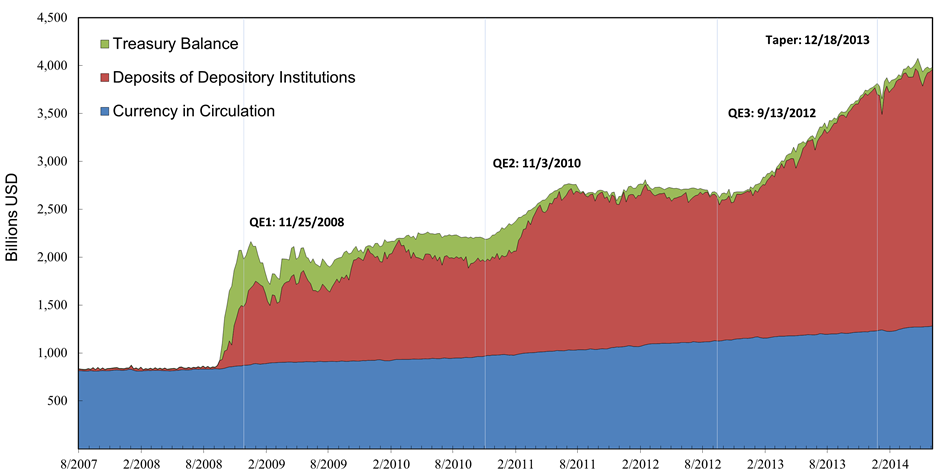
The question I originally asked was: do these excess reserves (as I have defined them) pose an inflationary threat when the economy returns to "normal?"

Inflationary Risk

Let us think of  "returning to normal" as an increase in x (a return of optimism) which induces the interest rate to R >1. In this case, we are back to case 1, but with a lower value for z. So yes, as illustrated in case 1, if z is to remain at this lower level, the price-level will be higher than it would otherwise be. This is the sense in which there is inflationary risk associated with "excess reserves" (in this model, at least).

Of course, in the model, there is a simple adjustment to monetary policy that would prevent the price-level from rising excessively. The Fed could just raise z (reverse the QE program).

In reality, reversing QE might not be enough. In the model above, I assumed that bonds were of very short duration. In reality, the average duration of the Fed's balance has been extended to about 10 years. What this means is that if interest rates spike up, the Fed is likely to suffer a capital loss on its portfolio. The implication is that it may not have enough assets to buy back all the reserves necessary to keep the price-level in check.

Alternatively, the Fed could increase the interest it pays on reserves. But in this case too, the question is how the interest charges are to be financed? If there is full support from the Treasury, then there is no problem. But if not, then the Fed will (effectively) have to print money (it would book a deferred asset) to finance interest on money. The effect of such a policy would be inflationary.

Finally, how is this related to bank-lending and private money creation? Well, in this model, where banks are assumed to intermediate all assets, broad money is given by M1 = D + P*k. We can eliminate P in this expression by using [16]:

[21] M1 = [ 1 + k/(y-k) ]*D

So when R > 1, reducing z has the effect of increasing capital spending and increasing M1. In the model, young agents want to "borrow" banknotes to finance additional investment spending. But it is not the increase in M1 that causes the price-level to rise. Instead, it is the reduction in the real demand for total government debt that causes the price-level to rise.

Likewise, in the case where R = 1 and then the economy returns to normal, the price-level pressure is coming from the portfolio substitution activity of economic agents: people want to dump their money and bonds in order to finance additional capital spending. The price-level rises as the demand for government securities falls. The fact that M1 is rising is incidental to this process.

Sunday, June 22, 2014

Excess reserves and inflation risk

Dave Wheelock, my colleague at the St. Louis Fed, points me to this nice article: Repeat After Me: Banks Cannot and Do Not "Lend Out" Reserves (by Paul Sheard). I have noticed a few papers lately making the same general point. I thought I'd throw my own two cents worth in.

To begin, you have probably seen (or heard about) this scary picture (thank you, "Helicopter" Ben):


That's a picture of the U.S. monetary base--the liabilities of the Federal Reserve Bank consisting of either currency or currency-on-demand (held by private, not government agencies). The monetary base can be divided into two broad categories: [1] currency in circulation (currency held by the non-bank private sector); and [2] reserves (bank sector vault cash and credits in reserve accounts held at the Fed).

In light of the "explosion" of Fed money since 2008, it may seem surprising that inflation has averaged considerably less than the Fed's official 2% target:


A common explanation for this is that most of the new money created by the Fed is being held by banks as reserves. Banks would rather earn 25 basis points (IOER) than lend out their excess reserves.

The following diagram depicts the liability side of the Fed's balance sheet:


We see that currency in circulation has increased, but at a modest and steady pace. Most of the increase in base money (remember, green part not included in money base) consists of reserves. The inflation fear expressed by some rests on the question of what is likely to happen once the economy returns to "normal." Sooner or later, things are going to turn around and banks will want to lend out their excess reserves to earn a higher rate of return. What is going to happen when this tidal wave of money begins to circulate?

According to Paul Sheard, this line of thinking is all wrong. That is, while monetary policy may ultimately result in higher inflation (or not), if it does, it won't be through the "banks lending out their excess reserves" channel, as many seem to suggest.

To understand his point, let's begin with how the Fed actually creates money. The Fed is a bank. And like all banks, it buys (or lends against) high-interest assets, which it finances by issuing low-interest liabilities (profits are returned to the Treasury). When the Fed buys a security on the open market, it credits the seller's bank account with newly-issued electronic digits (reserves). Banks then have the option of redeeming their reserves for currency, an option they may exercise depending on their customers' demand for currency.

Now, individuals regularly make deposits and withdrawals of cash into and out of their bank accounts. The net flow of withdrawals minus deposits determines by how currency in circulation grows over time. Banks do not lend out their cash. When a bank makes a loan, it issues a deposit liability that is redeemable for cash on demand. The demand deposit liabilities can be used as a payment instrument (they constitute money, and are counted as part of a broader measure of money supply, e.g., M1). The key observation here is that the way currency enters the economy is through the net withdrawal activity of bank customers--it has nothing to dow with banks lending out their reserves.

Alright, so why is understanding all this important? Well, for one thing, it is an accurate description of the way money and banking actually works (as opposed to the traditional "money multiplier" story that is commonly told in undergraduate textbooks). It is the right place to start when thinking of policy questions.

In terms of thinking about the inflation risk associated with the size of the Fed's balance sheet, it guides us away from examining how bank lending (the money multiplier) may react to various shocks. Banks can try to lend out their reserves all they want (create new loans). But if the public is satisfied with their currency holdings, any money injected into the system in this manner would have no effect on bank sector reserves. Since it is bank customers that determine how much cash is withdrawn from reserves, we should instead think about the type of shocks that may potentially alter this redemption decision.

To begin, we have to think about a world in which the asset side of the Fed's balance sheet matters. In many macroeconomic models, it is implicitly assumed that the Fed has full support of the Treasury (e.g., lump-sum taxes can be used to drain the economy of excess money), so that the Fed balance sheet does not matter. We want to do away with that assumption. In this case, the only "money draining" tools available to the Fed are asset sales. That is, think about the asset side of the Fed's balance as a giant vacuum cleaner. The amount of power this vacuum has is related to the market value of the Fed's asset portfolio. Any shock that would significantly reduce the market value of the Fed's asset portfolio would be like having your vacuum cleaner malfunction (just when you needed it the most).  


So, what type of shock can we think about here that might lend credence to the idea that excess reserves pose an inflation threat? I'm not really sure, but maybe the story goes something like this. Suppose that inflation expectations suddenly become "unanchored." (for whatever reason, people expect higher inflation). Through the Fisher equation, we might expect a large increase in nominal interest rates. The spike in interest rates would imply a capital loss for the Fed. By how much? Consider this formula (an approximation):

1 ppt increase in interest rate = (average duration)% decline in asset price. 

The average duration of the Fed's asset portfolio is roughly 10 years. So a five percentage point increase in interest rates would induce a 50% decline in the value of the Fed's assets (actually, somewhat less than this, but you get the point).

Now, higher inflation expectations on the part of the public may induce people to want to hold more currency (in nominal terms--the demand for real money balances may decline). This may be what could trigger a mass wave of redemptions. As people start withdrawing cash from their bank accounts, the banks start redeeming their reserves for cash to meet their customers' demands. The spike in interest rates unplugs the Fed's vacuum cleaner -- people know that the Fed does not have the tools to buy back all of its reserve liabilities. The wave of redemptions proceeds unchecked, with the flood of currency generating an inflation that becomes a self-fulfilling prophesy.

Well, that's just a story. I'm not sure if it hangs together logically (I've never seen it modeled formally, though perhaps it has been?) And even if it has a logical foundation, I'm not sure how persuasive it is. I am curious to know what other story one might tell. However the story unfolds, it cannot be one of bank lending out their reserves. 

Thursday, June 19, 2014

How far are we from trend?

I am always amazed at how well a log-linear trend line seems to fits real GDP (or per capita GDP) in the United States. Through a great depression, sandwiched by two world wars, secular changes in the relative importance of different sectors (agriculture, manufacturing, services), the baby boom, the increase in female labor force participation, etc. Through it all, the U.S. economy just seems to revert to the same log-linear trend. Maybe it was just a fluke. Whatever the case may be, that trend seems to have broken down since the great recession. We've all seen the diagram (the red line in the graph below -- thanks to my colleague Fernando Martin for the nice pictures).


The red line above plots the real GDP per capita (log scale) since 1955. The trend line is calculated over the sample period 1955-2007. The average growth rate is 2.2% per annum. You can see the big "output gap" emerging in 2008.

But given what we know about U.S. demographics--in particular the large rise, then fall in labor force participation, is the red line really the best way to look at things? A rough way to control for demographics is to consider the real GDP as a ratio of the labor force, instead of population. That is what the blue line does above. Once again, the trend line is computed for the same period 1955-2007. The average growth rate here is 1.5% per annum. What this tells us is that a lot of our measured growth over this period was due to nonstationary labor force behavior, and not just productivity. Oh, and the output gap near the end of the sample is considerably smaller. (It is too small to the extent that the recent decline in the labor force is attributable to "discouraged workers" who plan to return once conditions improve.)

Here is the same analysis for Canada:


The average growth rates are 1.7% (red) and 0.9% (blue), per annum. The blue line suggests that the Canadian economy is right on trend.
 
I think it's instructive to compare the U.S. to Canada. Consider, for example, the employment-to-population ratio for males aged 25-54:


There is a modest secular decline in the employment ratio in both countries.The Canadian employment ratio is currently not too far from its historical average, while the U.S. number still has some way to go. Of course, the great recession hit the U.S. much harder than Canada. Canada's great recession began in 1990 and it took about a decade for that economy to recover.

I began thinking about the similarity of the recent U.S. experience with Canada's earlier experience in this post: The Great Canadian Slump: Can it Happen in the U.S.? I followed up with a cross-country comparison of labor market behavior through the two episodes here: Employment Slumps in Canada and the U.S. Let me update the data there for males aged 25-54:


If the Canadian experience through the 1990s (red line) serves as a guide, then employment growth in the U.S. (blue line) will remain in recovery mode for another 4 or 5 years. While much of the gap has already been filled (it is not as dramatic as the first diagram suggests), there is still a considerable way to go when one looks at employment (instead of unemployment). So perhaps we are closer, but not as close to our goals as Jim Bullard suggests here: A Tame Taper.

Sunday, May 18, 2014

G and I in Europe and Japan

Izabella Kaminska reports here on a Credit Suisse comparison of Japan and the Euro area (h/t Scott Sumner). Here is an interesting diagram from that report:


According to Kaminska:
As the analysts note, a powerful fiscal stimulus in Japan helped to counter the demand shortfall. That caused personal consumption to continue to grow until 1997 and investment to rebound almost to its previous peak in just six years — something which isn’t slated for Europe any time soon.

Well, the increase in G counteracting an unexplained decline in I is one interpretation. This is the "deficient demand" interpretation that so many like to portray as obvious. But in fact, it's difficult to ascertain the direction of causality from just a picture.

The Japanese data above corresponds to what I posted some time ago here: What's Up with Japan? In response to that post, Mark Sadowski alerted me to the fact that the Japanese investment series plotted above includes both private and government spending. Here's what things look like when we decompose this aggregate (I discuss in more detail here: Another look at the Koizumi boom):


So it seems that there was a boom in private investment during the Koizumi years (something that Krugman gets wrong here, and something I'm not sure he's acknowledged). Moreover, this boom coincided with a slowing or outright contraction in government purchases. And in a liquidity trap era, I might add! What do our conventional "deficient demand" theories have to say about this? Maybe there is something more complicated than a simple IS-LM+liquidity trap story going on? I'm just asking. Humbly yours, DA.

Wednesday, March 26, 2014

Employment Along the Canada-U.S. Border (Part 2)

This is a follow-up to my earlier post: Employment Along the Canada-U.S. Border. In that post, I reported employment ratios and participation rates for three regions: Canada, U.S. states that bordered Canada, and U.S. states that did not border Canada. The main conclusion was that U.S. border states behave a lot more like non-border states, than they do Canada.

In this post, I (well, my fine research assistant, Lily, actually) report the same data but controlling for age and sex. In particular, I restrict attention to "prime age" workers--the age range 25-54 years old. I also divide the groups by sex. Here is what we get.


Participation rates for prime-age males has been declining steadily over time, but the decline seems to be much more dramatic in the U.S. Again, the border states follow their southern, rather than northern, counterparts.


The declining participation rates among men have been offset in part by the rising participation rates among prime-age women. Since about 2000, the participation rate among Canadian prime-age women continues to rise and remain stable, while in the U.S., the participation rate declines a bit. Again, the border states look more like their southern counterparts.


The great Canadian slump is evident in the 1990s. By the early 2000s, the employment to population ratio of prime-age males in both countries were roughly the same. The most recent recession hit the U.S. more severely than in Canada. Again, note that the border states followed their U.S. counterparts more closely than their Canadian neighbors.


According to this data, Canadian prime-age women were hardly affected by the recent recession.The pattern here is similar to the labor force participation rates described above.

While we can't say for sure just by looking at this data, I suspect that national policy differences are driving much of the different behavior here. But before I start looking for what these policy differences might be, I'll ask my trusty R.A. to look at sectoral decompositions.

Friday, March 21, 2014

Inflation expectations and real treasury yields

My colleague Kevin Kliesen supplies me with the following updates on inflation expectations and real treasury yields.

The first two plots show not very much action since the beginning of the year. The latest data show a recent tick down in inflation expectations, and a tick up in real yields:


Here is what the data looks like since 2007. Following some volatile behavior during the crisis, inflation expectations have roughly remained stable since 2009.


The interesting behavior since that time was fall yields and a flattening of the yield curve (nominal and real).  That downward trend appears to have reversed in mid 2013 (the taper tantrum), but has more or less remained stable since then (with the exception of the 2-year real, which has declined somewhat).

So while the real yield curve has steepened as of late, real yields are still well below where they were before the crisis (especially at the short end).

Friday, March 14, 2014

Employment Along the Canada-U.S. Border

I've written about differences in the Canadian and U.S. labor markets before; see here.  I see that Steve Williamson has recently chimed in as well with this: Why are Canadians Working so Much More than Americans?

A question that interested me is to what extent this cross-country difference is driven by regional considerations. That is, we know that most of the Canadian population lives and works near the U.S. border (the 49th parallel):


Now consider creating a new country consisting of U.S. border states: Washington, Montana, North Dakota, Minnesota, Wisconsin, Michigan, Ohio, New York, Vermont, New Hampshire and Maine (I exclude Alaska, Idaho, and Pennsylvania). If we were to combine these border states with Canada, the region of interest would look roughly like this (map is a little off, but you get the idea):


The question is this: Would you expect the labor market in the U.S. border states to look more like the Canadian labor market or more like the U.S. labor market?

There is good reason to believe, I think, that the demographics across the two countries are pretty similar (though certainly not identical). If the type of economic activity along the border is roughly similar across the two countries, then one might reasonably expect similar labor market behavior in Canada and the border states. But this is not what we see at all.

Here is a plot of the participation rate (employment plus unemployment as a ratio of the working age population):


The U.S. border states look a lot more like the rest of the U.S. and not like Canada at all. Here is a plot of the employment rate (employment as a ratio of the working age population):


Once again, the border states look more like the U.S. in general, rather than Canada.

A preliminary conclusion is as follows: [1] If Canada-U.S. demographics are roughly similar; and [2] if U.S. border states are roughly similar to their Canadian counterparts in terms of sectoral composition; then the differences we observe between the two countries (in terms of labor market activity) are quite possibly driven by policy differences.

Exactly what sort of policy differences we are talking about here remains an open question.