Believe those who are seeking the truth. Doubt those who find it. Andre Gide

Tuesday, November 23, 2010

The 2005 Real Wage Shock

In the course of preparing for my discussion of Rob Shimer's paper (see my post here), I had my RA (the tireless Constanza Liborio) dig up some aggregate wage data for the U.S. economy. Let me preface the discussion that follows by saying that I am wary of putting too much stock in aggregate wage data (the composition bias, in particular, is potentially a big problem; see here).  O.K., with this caveat in mind, let's take a look at some data.

As a measure of real wages, I use the BLS Employment Cost Index. Evidently, this measure is preferred by the likes of Bob Hall and others because it includes non-wage benefits. In what follows, I examine quarterly data for the sample period 1990:1 - 2010:3. The following chart plots the (annualized) rate of growth in nominal wages. The red line is a five-quarter rolling window I use to smooth out the series. The shaded areas represent NBER recession dates.


Prior to the most recent recession, nominal wages grew on average by about 3.5% per annum. The data shows a significant deceleration in nominal wage growth during the last recession. The composition bias suggests that actual wage growth displayed even greater "flexibility," as unemployment is typically concentrated among lower wage workers.

As I want to construct a measure of real wages, I need some measure of inflation. To this end, I use the GDP deflator, which is plotted in the next diagram.


Prior to the most recent recession, this measure of inflation averaged just above 2% per annum (the Fed's implicit inflation target). There was, however, a notable run up in the early 2000s, with (trend) inflation peaking at just over 3% in 2005 and early 2006. It is interesting to note that the rise in inflation over this period occurred while nominal wage growth decelerated. The next diagram plots the growth rate in real wages.


Now, the focus of Shimer's paper was apparent "ridigity" in real wage growth during the recent recession; a development that he interpreted as explaining the recent anemic behavior in employer recruiting intensity. As for myself, I was rather struck by the rapid deceleration in real wage growth in 2004, leading to falling real wages in 2005.

I want to take this data at face value for the moment and speculate a bit on what role these wage developments may have had in bursting of the U.S. home price "bubble" in 2006.

The story I have in my head revolves around an idea I first saw exposited by Joseph Zeira in his fine (and much under appreciated) paper: Informational overshooting, booms, and crashes

The basic idea in Zeira's paper is as follows. Imagine an asset whose dividend grows a H% per year. Everyone knows that this growth will one day come to an end. When this date arrives, the dividend grows at L% per year forever (a simplifying assumption), where L < H. The only uncertainty in this thought experiment pertains to the date of the "regime change."

Zeira demonstrates that the equilibrium (rational expectations) asset price rises over time, and continues to rise as long as dividend (read: real wage) growth expectations continue to be met. Then comes the shock.  I am tempted to call this a Wile E. Coyote moment, but of course, everyone in this model--unlike that hapless desert dog--knows that there is a date of reckoning. They just don't know beforehand when it will happen. So what happens?

Naturally, the asset price plummets like stone cast from heaven, before settling down along its new "fundamental" value (reflecting a new era of diminished expectations...gosh, I'm sounding a lot like PK these days). It appears as if asset prices "overshoot" their long-run fundamental value, before crashing.

To an outside observer, the asset price dynamics just described may be interpreted as a typical "irrational" boom and bust cycle (perhaps justifying some form of financial market regulation). In the context of the model world just described, this interpretation is completely wrong. This type of boom bust dynamic is, in fact, the natural consequence of how information is priced in an efficient asset market.

The picture I have in my head then is the following. Real wage growth appears relatively robust over the late 1990s and early 2000s. The return to labor, perhaps more than any other variable, measures the capacity for the average household to service debt. In the first half of the 2000s, creditors are looking at a recent history of relatively robust real wage growth, justifying credit expansion (even into subprime). By 2005, however, evidence of flagging fundamentals (anemic real wage growth) led to a (rational) revision downward in the real wage growth regime. Credit supply and real estate prices soon began to reflect this change in economic fundamentals.

Anyway, that's my crazy idea for the day. Feel free to share your thoughts...

Sunday, November 21, 2010

A Wile E. Coyote Moment

Paul Krugman has teamed up with NY Fed economist Gauti Eggertsson to produce a new working paper: Debt, Deleveraging, and the Liquidity Trap. Krugman provides a bit of background about this project on his blog. I see that at least a couple of people have already commented on paper; e.g., Nick Rowe and Steve Williamson. I thought that I'd join in on the fun.

And fun it is. Eggertsson and Krugman (henceforth, EK) certainly have a way with words. The imagery is splendid; my favorite, of course, being the Wile E. Coyote moment (or the Minsky moment) as reflecting the shock that unexpectedly slips the rug out from underneath the financial system.

O.K., so it's fun. But is it progress? I think it is. In particular, it's encouraging to see that the authors (Krugman, in particular, I suppose) are starting to take seriously the notion that agent heterogeneity and financial market frictions may be important elements to include in a theory of the business cycle. It should go without saying these latter two properties are the sine quibus non of modern macroeconomic modeling methodology.  As EK say in their abstract: "Making some agents debt-constrained is a surprisingly powerful assumption...". Yep, it's a real eye-opener alright. (For a few other surprises relating to the power of this assumption, see my entry here).

I want to keep this post reasonably short, so I limit myself to one (albeit important) aspect of the EK paper: the financial market friction, in the form of a debt constraint. Let me explain take a moment to explain the gist of it (for those who may be unfamiliar).

The key friction giving rise to this constraint is limited commitment (or limited enforcement). In lay terms, think about this as the unwillingness  to make good on one's promises. Taking out a loan would be no problem at all -- if debtors could be relied upon to honor their debt, in particular, by servicing it and paying it off out of their future earnings. But if debt default is a relatively low-cost proposition, then debtors may be tempted to exercise the option. To the extent that creditors anticipate these future default incentives, they are likely to restrict credit supply. The result is that people may not be able to get credit even if they are, in principle, able to pay it off.

As an aside, most people probably think of debt constraints as the consequence of "market failure" leading to an inefficiency. But as I explain here (A theory of inalienable property rights), legally imposed debt constraints might be the solution to a social problem when financial markets work too well. I mention this here because the social problem I highlight stems from heterogeneous time-discount factors, which is also a property of the EK model. In the absence of a debt-constraint, the impatient mortgage their future and embark on consumption trajectory that takes them to hell. Unfortunately for the rest of us, it is a hell that they share with the rest of society (a negative externality, in my model); so we prevent them from doing this.

Alright, back to the main story. So they have two types of agents in their model: patient and impatient. In an unfettered financial market, the latter are eventually enslaved to the former. But an exogenously imposed debt constraint prevents this extreme case from happening. Instead, the impatient hit their debt ceiling and then roll their debt over forever, paying interest to the creditors (the patient). If we call the patient agents "China" and the impatient agents "USA," we might start talking about "global imbalances." But let's not go there (though, if you're interested, you might want to go here).

And now for the Minsky moment: an unanticipated drop in the exogenous debt limit. The shock appears to be modeled as permanent. Imagine that a debtor is servicing a constant stock of $100 of debt (he'd like to borrow more, but creditors cannot secure themselves beyond $100). Following the Minsky moment, his debt limit is dropped to $75 (forever). Creditors are now worried that they cannot secure themselves beyond $75. So how does our debtor respond?

It seems to me that he will respond by defaulting on that portion of the debt he is able to; i.e., $25. I mean, why wouldn't he? It is not like he is committed to paying back debt; after all, the debt limit is rationalized in the first place by the limited commitment/enforcement friction.

And so, following a Minsky moment, we would expect a significant redistribution in wealth away from creditors toward debtors. Now that debtors have a lower cost of debt service, we can expect their consumption to increase (they are still debt-constrained, after all).

This is not, however, what happens in the EK model. Why not? Well, because following the Minsky moment, they impose the following behavioral assumption on debtors: "Suppose furthermore that the debtor must move quickly to bring debt within the new, lower, limit, and must therefore deleverage to the new borrowing constraint." [pg. 7]. Of course, this is what I assumed too. The difference is that EK assume that the deleveraging process does not entail default. Somehow, despite an implicit limited commitment friction, debtors are committed to deleveraging by paying down their debt. And, of course, paying down their debt means reducing consumption.

Is it not interesting how one is able to derive such polar opposite predictions from two plausible views of how debt is discharged following an unexpected financial market shock? Naturally, I am biased toward my view--not necessarily because it is descriptively more accurate (though we obviously do see defaults in the data) -- but because it appears logically more consistent with the frictions underlying the debt constraint in the model. If a prescribed behavior is inconsistent with the model environment, then (in my view) even more than the usual amount of caution is warranted in weighing the model's predictions and interpretation of events. (This is not to say that internal consistency is the only desired criterion of a model, of course.)

It would be interesting to explore the robustness of the EK results in the context of a model that takes the source of the debt limit (and its propensity to change) more seriously. (Not that the other shortcuts they take deserve any less attention.)  All in all, I like the paper because it at least makes at some attempt to formalize a popular interpretation of recent economic events. It's a small step forward and should, I think, spur a lively debate and future refinements...which is what our science is all about.

Thursday, November 18, 2010

Wage Rigidities and Jobless Recoveries

I recently attended an interesting conference hosted by the Atlanta Fed on Employment and the Business Cycle, where I had the pleasure of discussing this paper by Rob Shimer: Wage Rigidities and Jobless Recoveries. This was a fun paper to read, and I learned something new and interesting.

The backdrop for the paper is, of course, the recent financial crisis and associated recession. The level of GDP has essentially recovered its pre-recession level, while employment appears not to have recovered at all--these joint dynamics are referred to as a  "jobless recovery."

The hypothesis Shimer puts forth is this: [1] there was a shock (or shocks) that led to an evaporation in the value of the economy's capital stock; and [2] real wage growth is "sticky" in the sense that it appears insensitive to macro shocks.

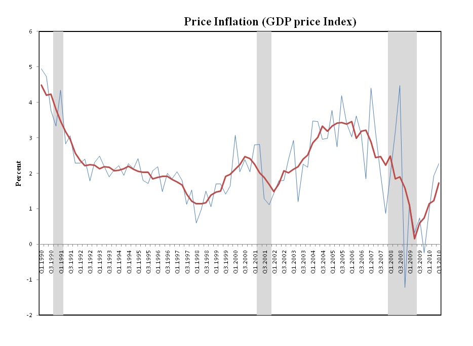
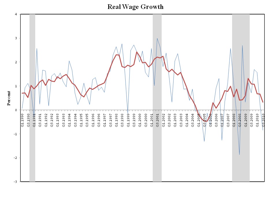
The type of evidence that lends some support for this latter hypothesis is displayed in the following diagram (also used by Bob Hall in his talk).


As an aside, I personally do not find such evidence wholly compelling. First, I think that composition bias is a big problem in the aggregate data; i.e., the first people to be let go in a recession are the least productive. Second, I have personal experience in the construction sector that leads me to believe that actual wage flexibility is much greater than what is recorded in official statistics. But in any case, I'm not here to argue about the evidence; let me take it as a fact that real wage growth is "sticky" in the sense described above. (Note: the basic story goes through as long as the real wage is not perfectly flexible).

To begin, consider a standard neoclassical growth model and let us consider a point on along the balanced growth path, where output and wages are growing, and employment (per capita) remains fixed over time.

Now, imagine that we shock the economy by evaporating some fraction of its capital stock. The subsequent transition dynamics are familiar to macroeconomic theorists and there is no need to describe them in detail here. The important thing is that real wages initially fall (since labor productivity falls and wages are flexible) and that the economy eventually returns to its balanced growth path.

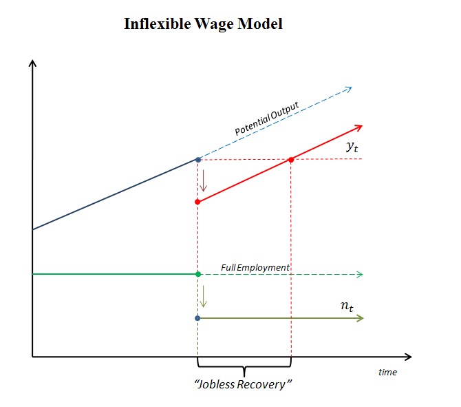
Next, let us repeat the experiment, but assuming instead that real wages continue to grow along their balanced growth path (that is, the real wage does not respond to the shock). What do the subsequent transition dynamics look like? My own expectation was that the economy would once again return to its balanced growth path, but that the period of transition would be extended owing to the assumed rigidity in the real wage. Everyone I quizzed about this had the same expectation.

Surprisingly, to me at least, this intuition turns out to be completely wrong! Output and employment drops on impact, but then output stays along its new balanced growth path, with employment remaining below full employment forever; see the following diagram.


Now, I have to admit that my first thought at reading this result was that it must surely be wrong. But, of course (this is Shimer after all), it turns out to be correct. You can verify this for yourself by reading the paper. But as this will probably take more effort than you're willing to expend, let me give you a much simpler example that conveys the basic intuition.

An OLG Model

People live for 2 periods and they value consumption only in the last period of life; write the utility function of a person born at date t as Ut = ct+1. This simplifying assumption implies that the young save all their income.

The young are each endowed with one unit of time, which they supply inelastically to the labor market. Let N denote the population of young workers; and assume that N remains constant over time. Let wt denote the real wage at date t.

The old are in possession of the economy's capital stock Kt. The old hire young labor at the prevailing wage, produce output, and then consume the profit (the return on capital). Capital depreciates fully after it is used in production.

There is a standard neoclassical production technology Y = F(K,N) satisfying Y = f(k)N, where k = K/N is the capital labor ratio. Let F be Cobb-Douglas and let 0 < α < 1 denote capital's share of output. Then we have f '(k)k = αf(k).

Now, the demand for labor satisfies: wt = FN(Kt,Ntd) and the supply of labor satisfies Nts = N. In a competitive equilibrium, the real wage must satisfy:

[1] wt = FN(Kt,N) = (1 - α)f(kt); where kt = Kt/N.

In what follows, I set the exogenous growth rate to zero, since doing so is not important for explaining the main result. Now, as the young save all their earnings, it follows that the next period capital stock (per young person) is given by:

[2] kt+1 = (1 - α)f(kt)

In other words, the dynamics are equivalent to the standard Solow model we teach to undergrads. The nondegenerate steady state capital-labor ratio is characterized by:

[3] k* = (1-α)f(k*)  [Note that k* = w* ]

Alright then. Begin at a point on the balanced growth path (here, a steady state with zero growth) and evaporate some capital, so that K0 < K*. This is a crude way to model the impact effect of a financial crisis. The transition dynamics should be familiar to any student of the Solow model; in particular, see [2]. In a decentralized version of this model, employment remains fixed at N, but the real wage (and the real wage bill) initially declines, before transitioning back to their original steady state values.

O.K., now let's repeat this experiment, but this time under the assumption that the real wage remains fixed at its initial steady-state value, wt = w* for all t. In this case, the level of employment N < N is determined the demand for labor; i.e.,

[4] w* = FN(K0,N0) = (1 - α)f(k*) = k*

Condition [4] implies that the capital-labor ratio remains unchanged; i.e., K0/N0 = k*. That is, the demand for labor declines in proportion to the decline in the value of capital. Since the real wage is fixed, this also implies that the aggregate wage bill declines in the same proportion. And since the wage bill here constitutes the saving that finances new capital, we have:

[5] K1 = w*N0 = K0 [since N0 = K0/k* and k* = w* ]

In other words, the capital stock remains forever fixed at K0 < K* and the level of employment remains forever fixed at N0 < N.

This is a permanent depression! If we extend the model to allow for exogenous growth, the level of employment remains depressed, but the level of output grows and eventually recovers its original level (this is the jobless recovery phase). However, the level of output remains forever below its "potential." Interesting.

Labor Market Search
 
One of the drawbacks of the model above is that both firms and workers stand to gain by negotiating the real wage downward following the shock. There is nothing in this model that prevents agents from exploiting these gains from trade, so ruling it out exogenously seems wrong (even if it is deemed realistic).

To address this shortcoming, Shimer extends the neoclassical model with the competitive labor market replaced by a search market, with bilateral meetings and negotiations. One of the nice things about the search specification is that the real wage may remain fixed in an equilibrium (if the shock is not too large). In other words, there need not be any inefficiency associated with a fixed wage at the individual level (though, it may induce an inefficiency at the aggregate level).

Shimer shows that the search model with rigid real wages generates dynamics that closely resemble those generated by a standard neoclassical model with rigid real wages. There appears to be an added force at work in the search model though. In particular, the combination of the negative shock and fixed real wage (along its balanced growth path) serves, in a way, to redistribute bargaining power from firms to workers. This is bad news for job creation, because the returns to investing in recruiting activities is now diminished, leading to a prolonged decline in employment. Sounds familiar.

In my view, this is an argument that deserves to be taken seriously. How seriously depends on how seriously one takes the "rigid real wage" hypothesis. Christopher Pissarides has criticized the assumption on the grounds that, in reality, real wages for new hires (or job changers) appear to be quite flexible relative to workers who remain employed. And, as Pissarides points out, the wages of incumbent workers do not factor into hiring decisions in a search model (assuming that the firm is not credit constrained). The key price as far as recruiting is concerned is the expected wage demands of future employees; and these appear to be relatively flexible.
 
This is all very interesting stuff. Almost makes me want to work in the area again!

P.S. The policy implications also turn out to be very interesting. Despite the "Keynesian" sticky wage property of these models, fiscal stimulus in the form of an increase in government purchases has the effect of crowding out capital investment, with no effect on employment. On the other hand, fiscal policies that subsidize business sector hiring (like a cut in the payroll tax) appear to be effective.

Wednesday, November 17, 2010

QE2 in Five Easy Pieces

A lot of people appear confused about QE2 and the Fed has recently come under a lot of attack following its recent announcement. Well, maybe the following will help a bit.  James Bullard, president of the St. Louis Fed, recently delivered a speech on QE2 entitled QE2 in Five Easy Pieces. For those that are interested, you can view his presentation slides here.

Monday, November 8, 2010

Ron Paul on the Fed Again

I have to admit that I like listening to the little guy speak. My view of Ron Paul (and yes, I have read End the Fed, though I haven't had time to comment on it yet) is that he is a smart guy with good instincts and a good understanding of the events that have shaped monetary history in the U.S. and elsewhere. (This is unlike PK who, while also very smart, appears to have shaped his macroeconomic theory entirely on the apparent failure of a local babysitting cooperative).

Here is Ron Paul's attack on the Fed today: Fed Will Self-Destruct. I don't necessarily disagree with any of the points made in the written article (apart from the fact that Bernanke has never advocated 4% inflation). Some of the things he says in the video interview, however, seem rather strange.

With respect to our "deeply flawed monetary system" he appears to be concerned that one person (Bernanke) has the power to create $600B with the stroke of pen (out of thin air) and then spend it (foolishly).

Note: while the Fed is indeed able to create cash (or reserve balances) "out of thin air," under normal circumstances, the Fed is effectively prevented from spending this cash on anything other than U.S. government bonds. These bonds are also created "out of thin air" (they exist almost exclusively in book entry form). When the Fed purchases government bonds, it is really just swapping one form of air for another.

When phrased in this way, it becomes a little harder to see why a swap of Fed air for Treasury air should be inflationary (though note, his definition of inflation is money creation -- so of course he sees inflation everywhere, even though price-level inflation remains anemic).

Wednesday, November 3, 2010

What is Clear and Not so Clear About Fed Policy (Part 2)

Today's FOMC statement is available here: FOMC November 03, 2010. Thought it might be a good time to follow up on my earlier (September 23) post: What is Clear and Not so Clear About Fed Policy.

On September 23, I said the following (let me summarize):

What was clear: The Fed will stand ready to do "whatever it takes" to make sure inflation expectations remain anchored at around 2% per annum. With inflation still on the low side of this target and the labor market still weak, it is not surprising that the Fed today a program to expand the size of its balance sheet.

What was not so clear: The Fed was not clear on the tactics it meant to employ to anchor long-term inflation expectations. I suggested that a good bet would be a program designed to purchase longer-dated treasuries, with purchases following a state-contingent rule (depending on how economic events turned out). This is what we got:
To promote a stronger pace of economic recovery and to help ensure that inflation, over time, is at levels consistent with its mandate, the Committee decided today to expand its holdings of securities. The Committee will maintain its existing policy of reinvesting principal payments from its securities holdings. In addition, the Committee intends to purchase a further $600 billion of longer-term Treasury securities by the end of the second quarter of 2011, a pace of about $75 billion per month. The Committee will regularly review the pace of its securities purchases and the overall size of the asset-purchase program in light of incoming information and will adjust the program as needed to best foster maximum employment and price stability.
Well, looks like I was half right. What surprised me here were the stipulated size and time limits; i.e., $600B figure by 2011:Q2. Why $600B and not $500B or $700B? No idea. Why 2011:Q2 and not 2011:Q1 or 2011:Q3? No idea.

The coexistence of the "state-contingent" and "size/time limit" language in the statement above may reflect a possible compromise between groups arguing for one or the other. But the "size/time limit" language seems somewhat redundant in my view; at least, given that we believe that the Fed is commited to 2% inflation. For example, what happens at the end of 2011:Q2 if inflation is still running at 1% with unemployment near double digits? Answer: a likely repeat, going further out along the yield curve, if necessary. But this is likely to happen (under the hypothesized contingency) whether or not these size/time limits were in place to begin with.

Finally, what was downright blurry in my previous post continues to remain hazy, in my view.

Tuesday, November 2, 2010

Bumper Stickers: Election 2010

Pretty much sums up the mood of the country, I'd say... (I saved the best one for last).